Achieving automation in sulfuric acid production relies heavily on PID control. However, in actual production, many valves remain manually operated. This is primarily due to technicians lacking experience in PID tuning, resulting in suboptimal parameter settings. This article shares a common tuning method—the empirical approach—to help address such challenges.

1. Empirical Method Tuning in Industrial Systems

The empirical method assigns suitable parameter ranges for controllers based on the nature of the controlled variable. This widely used tuning approach categorizes control systems by parameters such as level, flow, temperature, and pressure. Systems within the same category often share similar characteristics, allowing mutual reference for controller types and tuned parameters in most cases. Below, I analyze several common systems to help readers quickly grasp their distinct properties.

① Flow Control: Flow control is a typical fast process, often exhibiting noise due to turbulence, control valve oscillations, etc. For such processes, selecting a PI controller with a large proportional gain and short integral time is reasonable.

② Level Control: For applications requiring only average level control, pure proportional control with a large proportional gain is sufficient.

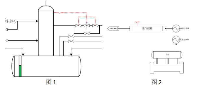
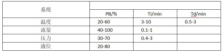
③ Pressure Control: Pressure loops can operate either very quickly or very slowly. For instance, Figure 1 shows direct control of the deaerator pressure point PI_1485, which exhibits extremely rapid response characteristics similar to flow control. Controller selection and parameter tuning can reference typical flow control practices. Figure 2 illustrates the steam pressure PI_1407 of the steam header, where both dynamic lag and flow lag inherent to the system are incorporated into the pressure control. These are influenced by pipeline length and volume, and parameter tuning can be referenced from temperature control practices.

④ Temperature Control: For the inlet temperatures of each converter section, thermal mass lag and heat transfer lag exist, resulting in slow response on the feedback display. Adding a small proportional gain is recommended. Selecting PID or PI control is reasonable.

Additional curve response experience can assist in tuning, requiring the introduction of the concept of pure dead time. The pure dead time refers to the time interval between the controller output (MV) changing and the process variable (PV) beginning to change. For a first-order controlled object with zero pure dead time, under purely proportional control, the control curve demonstrates: regardless of the proportional gain value, the closed-loop system remains stable without overshoot or oscillation. For systems with large dead time, a very small proportional gain is required to prevent oscillation in the setpoint step response. The optimal proportional gain of a pure proportional controller is inversely proportional to the system's dead time. When in-phase oscillations occur in the control loop (maximum and minimum values appear simultaneously on both lines, as shown in Figure 3), halving the proportional action can effectively improve closed-loop performance.

Empirical tuning parameters can be referenced from the table below, which meets the tuning requirements for most systems. If further fine-tuning is needed, initial values are typically provided. In temperature control systems where the controlled object directly absorbs radiant heat and exhibits high thermal conductivity, enabling rapid heating, the reference system often selects flow rate rather than temperature. In such cases, the flow system better describes these fast-process characteristics. Therefore, it is more accurate to understand the four systems described above as models.

These parameters provide field technicians with an empirical reference range. After determining the range based on system characteristics, parameters should be fine-tuned through trial and error.

2.External Manifestations and Limitations of Empirical Parameter Tuning

Many field commissioning engineers encounter situations where, after initially tuning loop parameters to a satisfactory curve, noticeable oscillations reappear over time. This typically indicates suboptimal curve tuning parameters, potentially triggered by load changes or external disturbances causing significant curve fluctuations. Theoretically, well-tuned parameters exhibit four key characteristics: First, during step responses (sudden setpoint changes), the system must respond rapidly, with overshoot remaining within process tolerance limits and achieving swift stabilization. Second, the system should recover quickly to the setpoint after external disturbances. Third, the manipulated variable (MV) should exhibit smooth behavior; its corresponding curve on the DCS should show no abrupt jumps. Fourth, robust performance must be maintained across varying operating conditions.

Empirical tuning is a common approach among field technicians, but relying solely on experience as a universal solution is unrealistic. For instance, empirical methods become ineffective when loops exhibit coupling effects. In such cases, applying conventional tuning methods reveals that changes in one loop affect another. This necessitates decoupling and tuning each loop separately. Each situation requires specific analysis—there is no perfect PID, only the appropriate PID.